by Ben-chin K Cha
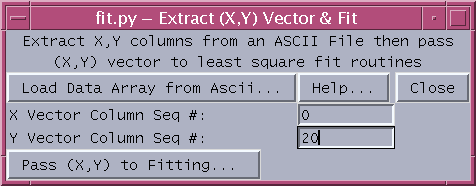
The user interface is implemented through using python Tkinter and Pmw widgets. It allows the user freely to load the desired Ascii file and extract the desired vector to be fitted. It is assumed that column oriented data array defined in text file. Any line start with ';' or '#' will be treated as comment and ignored. The Ascii file may or may not contain independent variable vector.
Zero based index sequence number is used in indexing the X and Y vectors. By default it assumed that column oriented vector array defined in the text file and the first column (0) contains the X vector. The remaining columns starting from the second column (1) contain the dependent variable vectors. User can easily to pick the desired Y vector from the column array by entering the column sequence number for Y vector.
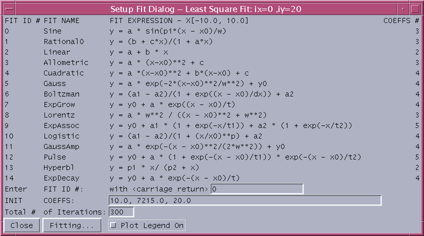
At present the following set of fit functions available in fit.py for least square fit of the selected Y vector:
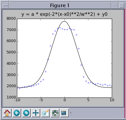
	Polynomial Fit 	- y = a0*x**n + a1*x**(n-1)+...+ an
	Sine Fit	- y = a*sin(pi*(x-x0)/w)
	Rtional0 Fit	- y = (b+c*x)/(1+a*x)
	Linear Fit	- y = a + b*x
	Allometric Fit  - y = a*(x-x0)**2 + c
	Cuadratic Fit	- y = a*(x-x0)**2+b*(x-x0)+c
	Gauss Fit	- y = a*exp(-2*(x-x0)**2/W**2)+y0
	Boltzman Fit	- y = (a1-a2)/(1+exp((x-x0)/dx)) + a2
	ExpGrow Fit	- y = y0 + a*exp((x-x0)/t)
	Lorentz Fit	- y = a*w**2/((x-x0)**2+w**2)
	ExpAssoc Fit	- y = y0 + a1*(1+exp(-x/t1))+a2*(1+exp(-x/t2))
	Logistic Fit	- y = (a1-a2)/(1+(x/x0)**p)+a2
	GaussAmp	- y = a*exp(-(x-x0)**2/(2*w**2))+y0
	Pulse Fit	- y = y0 +a*(1+exp(-(x-x0)/t1))*exp(-(x-x0)/t2)
	Hyperbl	Fit	- y = p1*x/(p2+x)
	ExpDecay Fit	- y = y0+a*exp(-(x-x0)/t)
Please refer the fit.html for avaialbe functions or methods defined in fit.py.
| pviewer.zip | (0.126MB) | A collection of 1D/2D/3D graphic programs for python package |
	Tkinter		- Tk user interface
	Pmw		- python mega widgets
	matplotlib	- python matlab plot library
	Numeric		- python numeic  package
	numarray	- python numarray  package
	Pygtk		- python GTK package
	Scientific	- python scientific package
	source /APSshare/setup_apsshare
	fit.py
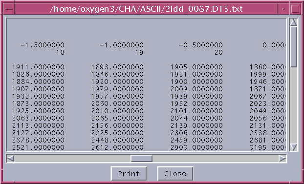
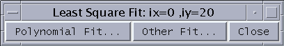
Following interface windows show primary result of loading data from Ascii text file. The active plot window can be easily closed by simply clicking the right mouse button on the plot area. The configuration file fit.config is used for easy restart of fit.py.
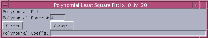
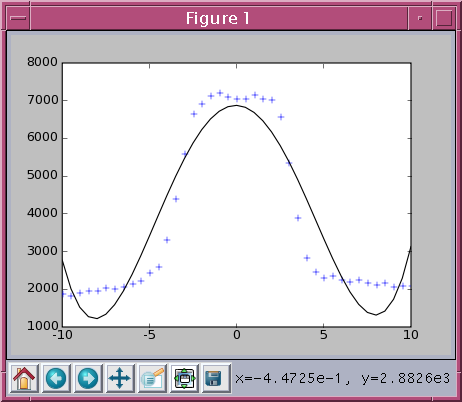
Follwing figure show the resullt of polynomial fitting with power of 4.
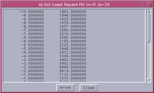
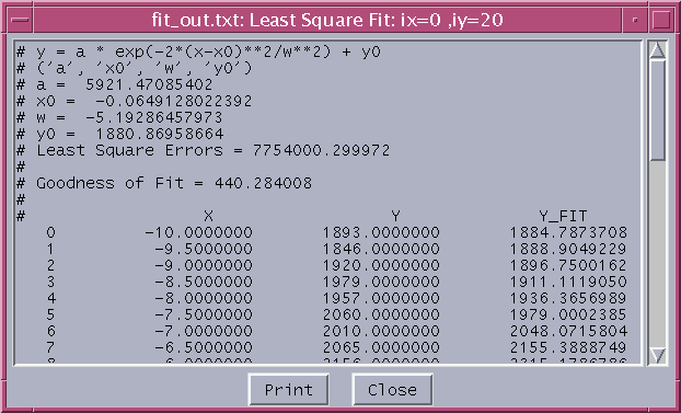
Following figure shows the tabulated text result of 'Gauss' Fit.
Following figure shows the plot result of 'Gauss' Fit.